Code
## Some contants to use later

# Air density at sea level
RHO = 1.225 # kg/m3
# Gravitational accel
GRAV = 9.8 # m/s2
# Convert meters per second to miles per hour
MPS_TO_MPH = 2.237
# Convert LB to KG
KG_PER_LB = 0.4536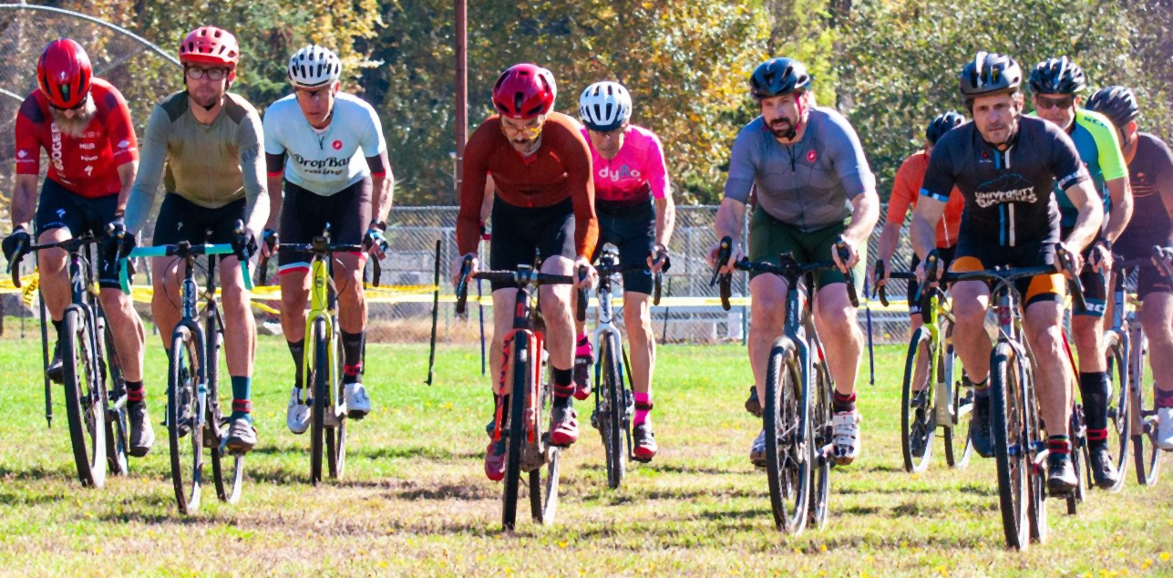
In a cyclocross race, there are a lot of tight corners – often muddy – which force you to slow down to a near stop. There also tend to be quite a few straight flat sections where you can go fast. These vary in length a lot – but sometimes they can be quite long (hundreds of meters). It occurred to me at a race recently that it’s probably valuable to pedal as hard as you can at the start of these sections, even if that means you have to take it easier for the rest of it, because you get to ride that momentum for longer. In other words, a joule put out at the beginning is a lot more valuable than a joule near the end, because the joule at the end is just going to go immediately into your brakes as you hit the next corner.
Intuitively, this seemed obviously correct, but I wanted to quantify just how much difference it could make! To do that, I went searching for some estimates for things like rolling resistance, and then wrote a little physics simulation to try out different scenarios. For this post, I’m going to measure the time difference for an 80-meter straight-away between two scenarios where an equal amount of energy is applied. In one scenario, the rider puts out constant power throughout the straight. In the second scenario, the rider puts out a burst of higher power for a few seconds, and then backs off the power to a lower value, chosen so that the total energy put out is equal in both cases.
Additionally, since we’re here, we’ll look at how much power is lost to aero drag vs rolling resistance relative to the power that goes into kinetic energy (and ultimately probably your brakes), and whether the rotational momentum of the wheel actually matters.
Rotational inertia of the wheel barely matters at all
## Some contants to use later
# Air density at sea level
RHO = 1.225 # kg/m3
# Gravitational accel
GRAV = 9.8 # m/s2
# Convert meters per second to miles per hour
MPS_TO_MPH = 2.237
# Convert LB to KG
KG_PER_LB = 0.4536First, I need to estimate the parameters required to model the following factors:
I’m going to just ignore drive train efficiency. There is also a question of human body efficiency – i.e., I don’t necessarily believe that the fatigue experienced by a rider (however that is quantified) is truly proportional to total energy output, but I hope comparing equal energy efforts is reasonable here.
I made a rough estimate of the moment of inertia of my wheels by weighing one of the heavier ones and then just assuming that all of that mass is at the rim radius. It’s rough, but as we’ll see later this doesn’t really matter.
My wheel measured 1.8kg on a scale. The rim radius on 700C wheels is 311mm. The moment of inertia for each is calculated as \(I = mr^{2}\), and I multiply that by two to account for both wheels.
# Moment of inertia is mass * radius^2
Iwheel = 2 * 1.8 * 0.311**2 # kg * m2

# Wheel radius is to the outside of the tire
#
# This can vary a lot, based on the tire and the pressure. I measured my Challenge TLR 38mm to get
# this value.
wheel_radius = 0.362 # metersThis is simply \({{1} \over {2}} mv^{2}\), so all we need to know is the mass, \(m\). This of course has to include the rider. I just used my own weight (185lb) and bike weight (18lb).
# Bike mass
bike_mass = (185 + 18) * KG_PER_LB # kg
Rolling resistance is the force created mainly by the inelastic displacement of your tire and/or the ground under your tire. The force is actually a constant for us, as it depends only on the coefficient of rolling resistance \(C_{RR}\) and the normal force, which depends on just mass and gravity. The power loss is \(P = Fv\), so it increases proportionally with velocity.
So, the power lost to rolling resistance is given by \(P_{RR} = C_{RR}mgv\), where \(m\) is mass in kg, \(g\) is the gravitional constant of 9.8 m/s, and \(v\) is velocity in m/s.
This is perhaps the hardest thing to estimate, because it depends on a lot of things. In addition to rider weight, it depends on the shape and material of the tire, the inflation pressure, and the ground your running on. I’m sure you can imagine the difference between rolling on pavement and sand – CX races have both!
For this, I am relying on Nick at morespeedlesspower.com for data. Nick did a bunch of well controlled testing, and it seems like the best source I could find. Most of the tire rolling resistance calculations our there are done on drums. Some of the tests have rough drums, to simulate gravel or whatever, but still, the drum itself is rigid and the ground we ride on a cyclocross course is often not at all rigid. Nick did testing with the right sort of tires, on grass, which is about as close to the circumstances I’m interested in as I can hope to get. At 30PSI, he measures Crr of 0.025 - 0.03. I’m splitting the difference. Thanks Nick for publishing this!
# Coefficient of Rolling Resistance
Crr = 0.0275 # dimensionlessThe power lost to aerodynamic drag is described by coefficient \(C_{d}A\), which has units of \(m^2\). The power lost is: \(P_{aero} = {{1} \over {2}}C_{d}A{\rho}v^{3}\), where \({\rho}\) is air density (\(1.225 kg / m^{3}\)) and v is velocity in m/s.
There are lots of sources out there for this – it’s a lot less variable and easier to measure. Nick from above, for example, measured his \(C_{d}A\) at \(0.393m^{2}\).
gymcreek.com suggests a range of \(0.31-0.4m^{2}\) when “on the hoods”.
I decided to go with something in the middle of that.
# Aero drag
Cda = 0.35 # m^2The simulation is run as a simple differential equation, using kinetic energy and distance as variables. The system is run using scipy.integrate.solve_ivp. For the burst scenario, there are two different power outputs: \(P_{high}\) is applied for a few seconds, then \(P_{low}\) is applied until the finish line is reached. A root solver is used to iteratively search for the value of \(P_{low}\) which results in the same total energy expenditure as the constant power scenario.
The system is given by the following differential equations
\[ \begin{aligned} E' &= P_{in} - P{aero} - P_{RR} \\ d' &= v \end{aligned} \]
The rate of change in kinetic energy is just the input power from the pedals less the losses to aero drag and rolling resistance (described above). The rate of change in distance is velocity.
Velocity and energy are directly related by \(E = C_{i}v^{2}\), where \(C_i\) is a constant combining the rotational kinetic energy of the wheel and the translational energy of the bike and rider:
Rotational energy is \(E_{r} = {{1} \over {2}}I{\omega}^{2}\), where I is the wheel’s moment of inertia, and \({\omega}\) is the angular velocity of the wheel. We can replace \({\omega}\) with \({\omega} = {v \over r}\). Translational energy is \(E_{t} = {{1} \over {2}}mv^{2}\). The combined coefficient is then \({C_i} = {{1} \over {2}}m + {I \over {2r^{2}}}\)
The following code block implements the simulation itself. Feel free to tell me how I screwed it up if you like!
import matplotlib.pyplot as plt
import numpy as np
import scipy.optimize
import scipy.integrate
import seaborn as sns
sns.set_theme()
# # Combined coefficient of inertial
#
# The bike stores kinetic energy in two places:
# - The wheel's rotation energy E_r = 0.5 * I * w^2
# - The translational energy E_t = 0.5 * mass * v^2
#
# The angular velocity of the wheel (w) is related to translational velocity (v) by w = v / r, where
# r is the wheel radius. So, E_r can be express as E_r = (0.5 * I / r^2) * v^2.
Ci = 0.5 * bike_mass + 0.5 * Iwheel / wheel_radius**2

def create_power_step_fn(Phigh: float, Thigh: float, Plow: float) -> callable:
    def f(t):
        result = np.where(np.asarray(t) < Thigh, Phigh, Plow)
        return result.item() if result.ndim == 0 else result
    return f

def get_aero_loss(v) -> float:
    """ Get aero loss in watts

    v: forward velocity in m/s
    """
    return 0.5 * RHO * Cda * v**3

def get_rolling_resistance_loss(v: float) -> float:
    """Get the rolling resistance power loss in watts

    v: forward velocity in m/s
    """
    return Crr * bike_mass * GRAV * v

def finish_threshold(distance) -> callable:
    """Create event function for simulation

    Event fires when distance (y[1]) exceeds threshold
    """
    def f(t, y):
        return distance - y[1]
    # end the simulation when event occurs
    f.terminal=True
    return f


def race_fn(power_step_fn):
    def f(t, x):
        E = max(0.0, x[0])
        d = x[1]

        # Compute velocity from system energy
        v = np.sqrt(E / Ci)

        # Compute power lost to aero drag
        Paero = get_aero_loss(v)
        # Compute power lost to rolling resistance
        Prr = get_rolling_resistance_loss(v)

        Pin = power_step_fn(t)
        Pnet = Pin - Paero - Prr

        return [Pnet, v]

    return f

class SimResult(object):
    def __init__(self, t, Pin, Paero, Prr, v, d):
        self.t = t
        self.Pin = Pin
        self.Paero = Paero
        self.Prr = Prr
        self.v = v
        self.d = d

    def finish_time(self):
        return self.t[-1]


def run_simulation(Phigh: float, Thigh: float, Plow: float, distance: float) -> SimResult:
    power_fn = create_power_step_fn(Phigh, Thigh, Plow)
    sol = scipy.integrate.solve_ivp(
        race_fn(power_fn),
        (0, 1000),
        (0, 0),
        events=finish_threshold(distance),
        rtol=1e-7,
        atol=1e-9,
    )

    if not sol.success:
        raise RuntimeError(f"Simulation failed: {sol.message}")

    E = np.clip(sol.y[0], min=0.0)
    d = sol.y[1]
    v = np.sqrt(E / Ci)
    Pin = power_fn(sol.t)
    Paero = get_aero_loss(v)
    Prr = get_rolling_resistance_loss(v)

    return SimResult(t=sol.t, Pin=Pin, Paero=Paero, Prr=Prr, v=v, d=d)

def solve_for_energy(Phigh:float, Thigh:float, energy:float, distance:float=100) -> float:
    """Find Plow so the input energy at the 100 m finish equals ``energy``.

    The energy is Phigh * min(Thigh, Tfinish) + Plow * max(0, Tfinish - Thigh),
    where Tfinish is the time at which the simulation reaches DISTANCE.
    """

    if Phigh < 0 or Thigh < 0 or energy < 0:
        raise ValueError("Phigh, Thigh, and energy must be non-negative")

    def energy_error(Plow):
        result = run_simulation(Phigh, Thigh, Plow, distance=distance)

        finish_time = result.finish_time()
        high_duration = min(Thigh, finish_time)
        low_duration = max(0.0, finish_time - Thigh)
        consumed_energy = Phigh * high_duration + Plow * low_duration
        return consumed_energy - energy

    # Find two powers that reach the finish and bracket the requested energy.
    # Increasing Plow makes the finish happen sooner and the consumed energy
    # approach the energy required to finish with Phigh alone.
    bracket_low = None
    bracket_high = None
    low_error = high_error = None
    Plow = 0.0
    for _ in range(60):
        error = energy_error(Plow)
        if error is not None:
            if bracket_low is None:
                bracket_low, low_error = Plow, error
            if error == 0:
                return Plow
            if low_error * error < 0:
                bracket_high, high_error = Plow, error
                break
            bracket_low, low_error = Plow, error
        Plow = 1.0 if Plow == 0 else Plow * 2.0

    if bracket_high is None:
        raise ValueError(
            "Could not bracket a solution: the requested energy may be "
            "unreachable for this Phigh and Thigh."
        )

    def bracketed_error(power):
        error = energy_error(power)
        if error is None:
            raise RuntimeError("A bracket endpoint unexpectedly failed to reach the finish")
        return error

    return scipy.optimize.brentq(
        bracketed_error, bracket_low, bracket_high, xtol=1e-6, rtol=1e-8
    )
Here’s a scenario to compare! The scenario I’ve chosen is an 80-meter straight. In the constant power case, 300W is applied throughout the sprint. In the burst case, our simulated rider stands up and puts out 600W for just 4 seconds, then sits down and does 238W the rest of the way.
As shown in the plot below, both riders reach very nearly the same top speeds, but the second rider accelerates faster. The first rider takes 15.7 seconds to reach the next corner, 2 seconds after the rider who stood up. Maybe two seconds doesn’t sound like much, but I think this scenario happens dozens of times in a typical race, and at my last race the next guy was only 4 seconds behind me!
I think there’s also a tactical advantage because if you don’t come out of the turn hot, then it’s a great opportunity for someone to pass you!
DISTANCE=80

# Run a constant 200W case
CONSTANT_WATTS = 300
sol_constant = run_simulation(CONSTANT_WATTS, 1, CONSTANT_WATTS, distance=DISTANCE)
total_energy = CONSTANT_WATTS * sol_constant.finish_time()

# Run a case with early burst power
Phigh = 600 # Power during early burst
Thigh = 4 # Duration of early burst
Plow = solve_for_energy(Phigh, Thigh, total_energy, distance=DISTANCE)
sol_burst = run_simulation(Phigh, Thigh, Plow, distance=DISTANCE)

t1 = sol_constant.finish_time()
t2 = sol_burst.finish_time()
deltaT = t1 - t2

(fig, axes) = plt.subplots(2,1)
axes[0].plot(sol_constant.t, sol_constant.Pin, label="Constant")
axes[0].plot(sol_burst.t, sol_burst.Pin, label="Burst")
axes[0].set_ylim(bottom=0)
axes[0].set_ylabel("Pedal Power (W)")
axes[0].set_title(f"Power applied over {DISTANCE}m sprint\nEnergy (∫Pdt) is equal in both cases")
axes[0].tick_params(axis="x", labelbottom=False)
axes[0].legend()

axes[1].plot(sol_constant.t, sol_constant.v * MPS_TO_MPH, label="Constant")
axes[1].plot(sol_burst.t, sol_burst.v * MPS_TO_MPH, label="Burst")
axes[1].set_ylabel("Speed (MPH)")
axes[1].set_xlabel("Time (s)")
axes[1].set_title(f"T1 = {t1:.2f}s, T2 = {t2:.2f}s, ΔT = {deltaT:.2f}s")
axes[1].legend()

plt.tight_layout()
plt.show()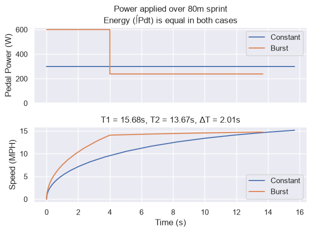
A potentially interesting follow-on question to ask is, “where is the input energy going?” There are basically three possibilities:
For the last point though, I was also curious where the energy is stored: how much is translational kinetic energy of your motion, and how much is rotational energy in the wheels?
You can see from the plot below first of all that almost no energy goes into the rotation of the wheels. This was a little surprising, because I’ve heard people talking about how “weight in the wheels is doubly important because they have to spin”. Well, no! It’s not anywhere near twice as important. In fact, it’s so small as to be virtually irrelevant. Actually, it’s easy to quantify by comparing the two terms of \(C_i\): Only 2.8% of the kinetic energy is going into the wheel rotation, and that is with some pretty heavy wheels, compared to most race wheels.
I wasn’t too surprised to see that rolling resistance dominates the losses on grass at these relatively slow speeds, but it’s nice to see just how much and to hone my intuitions.
# Integrate power to get energy
Eaero = scipy.integrate.cumulative_trapezoid(sol_burst.Paero, sol_burst.t, initial=0)
Err = scipy.integrate.cumulative_trapezoid(sol_burst.Prr, sol_burst.t, initial=0)

# Kinetic energy is just a function of velocity
Ewheel = (0.5 * Iwheel / (wheel_radius ** 2)) * (sol_burst.v ** 2)
Etrans = 0.5 * bike_mass * (sol_burst.v ** 2)

(fig, axes) = plt.subplots(1, 1)
axes.plot(sol_burst.t, Eaero, "-.", label="Lost to Aero")
axes.plot(sol_burst.t, Err, "-.", label="Lost to Rolling")
axes.plot(sol_burst.t, Ewheel, label="Rotational Kinetic")
axes.plot(sol_burst.t, Etrans, label="Translational Kinetic")
axes.legend()
axes.set_ylabel("Energy (Joules)")
axes.set_xlabel("Time (s)")
plt.show()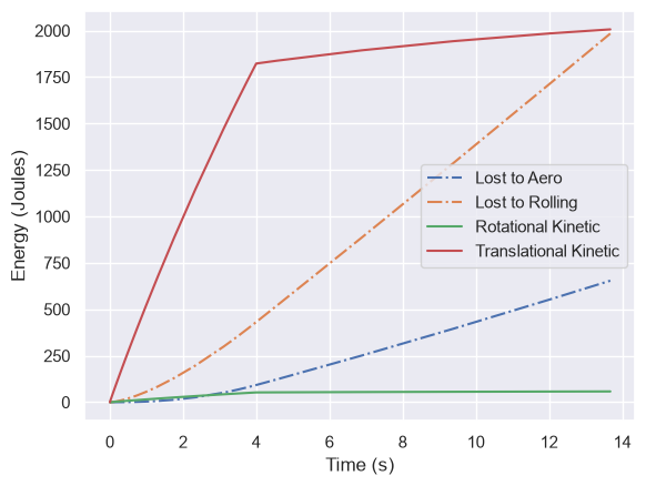
Just to be sure that the solver worked, and the total energy is equal in both scenarios, let’s integrate the input power:
print(f"Constant energy: {np.trapezoid(sol_constant.Pin, sol_constant.t):.1f}J")
print(f"Burst energy: {np.trapezoid(sol_burst.Pin, sol_burst.t):.1f}J")
print(f"Burst P_low: {sol_burst.Pin[-1]:.1f}W")
Constant energy: 4704.3J
Burst energy: 4704.4J
Burst P_low: 238.2WEven though you’re probably tired out there, stand up and dig deep immediately as you enter that long strait and I’m pretty sure it will pay off. Just a few good strokes, and then take your breather while you ride that momentum.
The main straight that inspired this line of thought and helped ot establish the 80m distance was at Steel Lake Park, and, as it happens, my race buddy Curtis filmed it! So if you want to get a better idea of it, check out his Youtube video at around 7:40. There’s a tight pair of corners which force you to slow way down, and then a long grass straight, and I think it’s funny that Curtis seemed to be thinking along a similar line at the same spot on the course.